A tutorial on analyzing ordinal data
A tutorial on analyzing ordinal data
September 2024
Introduction
Lately in my consulting practice, I have had many questions about analyzing ordinal data, that is, categorical data for which the categories can be ordered in a way that makes sense. For example, the “star system” you may have used to rate that restaurant you visited in Portland that took an hour to seat you, played music too loud to hear the conversation, and then charged absurd prices for mediocre small plates that left you still hungry at the end on some social rating platform is a type of ordinal scale. The star system yields ordinal data because a 3-star rating is greater/better than a two-star rating, but the data aren’t really numeric but rather categorical.
Indeed, it may be tempting to treat the data as numeric. After all, an average rating of 3.2 is greater than an average rating of 2.7. However, treating the data as numeric implicitly assumes that 2 is exactly one unit greater than a rating of 1 and one unit less than a rating of 3, and that a 5 is still only one unit better than a 4. But ask yourself, “is that really the way I rate restaurants?”. Personally, I might give a 4-star rating to any good restaurant, but I reserve a 5-star rating for the best of the best, which are way better than the good restaurants. Similarly, 1-star reviews are reserved for the bottom of the barrel and the difference between 1 and 2 stars is a lot greater than the difference between 3 and 4 stars in my mind.
Because of this unequal spacing issue, ordinal data get their own distinction and usually should not be treated as numeric unless well-justified by prior knowledge. But, how can we analyze such data? Below I present one option that is in line with a generalized linear modeling (GLM) approach.
Motivating example
Assume we have distributed a short survey to 100 people from each of two communities, one rural and one urban, and asked the respondents to rate three pictures of the same national park but taken at different locations in terms of how desirable each looks as a vacation destination. The first picture includes strictly “natural” scenery, the second includes some trails through meadows with some people hiking on them, and the last includes a gift shop and a welcome center with a stunning backdrop. The hypothesis is that people will gravitate towards the familiar, so those living in urban areas will rate the second two photos higher than the first since there are more signs of familiar human development in them, while people from rural areas will rate the photos with less evidence of human influence higher.
Important caveat: I am not a social scientist and am just making this stuff up! Forgive me if you are a social scientist and this is totally ridiculous 🙂.
A summary of these fictitious data is shown in Table 1.
| community | photo | mean_rating | n_respondents |
|---|---|---|---|
| rural | buildings | 3.10 | 100 |
| rural | natural | 4.59 | 100 |
| rural | trails | 3.97 | 100 |
| urban | buildings | 3.80 | 100 |
| urban | natural | 2.54 | 100 |
| urban | trails | 3.87 | 100 |
Table 1: Data summary.
Ordered Probit Model
With the ordered probit model, we imagine a normal distribution on a latent (i.e., unobserved) scale with mean equal to the linear predictor for observation \(i = 1,2,...,n\),
\[\eta_i = {\bf x}_i^\top \boldsymbol \beta\]and a variance of \(\sigma^2 = 1\). So far, this is simply multiple regression, we just don’t get to see this regression on the continuous scale. Instead, what we observe is a filtered version of the “true”, continuous observation (e.g., how appealing a given photo is to the respondent on a continuous, unbounded scale). Specifically, we define a set of \(K-1\) thresholds, \(\theta_1, ..., \theta_{K-1}\), where \(K\) is the number of categories in the ordinal variable (5 in our example). It is assumed that \(\theta_0 = -\infty\) and \(\theta_K = \infty\). The “filtering” process we imagine assumes that a realization from the normal distribution with mean \({\bf x}_i^\top \boldsymbol \beta\) and variance of 1, denoted \(y_i^*\), gets “binned” into the ordinal categories by the thresholds. So, for example, if \(\theta_{1} < y_i^* \le \theta_2\), then the respondent would provide a rating of 2 stars. If instead \(\theta_4 < y_i^* < \infty = \theta_5\), then the respondent would provide a rating of 5 stars.
Given this model, we define the probability that a given person with covariates \({\bf x}_i\) gives a rating of \(k\) as
\[P(\theta_{k-1} < {\bf x_i}^\top \boldsymbol \beta + \epsilon_i < \theta_k)\]where \(\epsilon_1, \epsilon_2, ..., \epsilon_n \sim \mathcal{N}({\bf 0}, \Omega)\) and \(\Omega\) is an \(n\times n\) correlation matrix (it’s a correlation matrix rather than a covariance matrix since we assume the errors have variance of 1). Given the data, we jointly estimate the parameters \((\boldsymbol \beta, \boldsymbol \theta, \boldsymbol \Omega)\), though it is most often assumed that the errors are independent such that \(\Omega = I_n\).
Fitting the model using brms
While there are a few R packages out there than can estimate ordered
probit models, brms (i.e., Bayesian Regression Models using Stan) is
the most flexible. Furthermore, it uses syntax to define models that
will be familiar to many R users and it is possible to use the posterior
predictions to check model fit. Here is an example using the fictitious
data described in Section 2.
library(brms)
library(tidyverse)

# ensure our variables are of the correct class
dat <- dat %>% mutate(
  photo = factor(
    photo,
    levels = c("natural", "trails", "buildings")
  ),
  community = factor(community),
  person = factor(person),
  rating = ordered(rating)
)

# fitting the model
mfit_init <- brm(
  rating ~ photo * community + (1 | person),
  family = cumulative(link = "probit"),
  data = dat,
  cores = 4
)
## Running /Library/Frameworks/R.framework/Resources/bin/R CMD SHLIB foo.c
## using C compiler: ‘Apple clang version 15.0.0 (clang-1500.3.9.4)’
## using SDK: ‘’
## clang -arch x86_64 -I"/Library/Frameworks/R.framework/Resources/include" -DNDEBUG   -I"/Library/Frameworks/R.framework/Versions/4.4-x86_64/Resources/library/Rcpp/include/"  -I"/Library/Frameworks/R.framework/Versions/4.4-x86_64/Resources/library/RcppEigen/include/"  -I"/Library/Frameworks/R.framework/Versions/4.4-x86_64/Resources/library/RcppEigen/include/unsupported"  -I"/Library/Frameworks/R.framework/Versions/4.4-x86_64/Resources/library/BH/include" -I"/Library/Frameworks/R.framework/Versions/4.4-x86_64/Resources/library/StanHeaders/include/src/"  -I"/Library/Frameworks/R.framework/Versions/4.4-x86_64/Resources/library/StanHeaders/include/"  -I"/Library/Frameworks/R.framework/Versions/4.4-x86_64/Resources/library/RcppParallel/include/"  -I"/Library/Frameworks/R.framework/Versions/4.4-x86_64/Resources/library/rstan/include" -DEIGEN_NO_DEBUG  -DBOOST_DISABLE_ASSERTS  -DBOOST_PENDING_INTEGER_LOG2_HPP  -DSTAN_THREADS  -DUSE_STANC3 -DSTRICT_R_HEADERS  -DBOOST_PHOENIX_NO_VARIADIC_EXPRESSION  -D_HAS_AUTO_PTR_ETC=0  -include '/Library/Frameworks/R.framework/Versions/4.4-x86_64/Resources/library/StanHeaders/include/stan/math/prim/fun/Eigen.hpp'  -D_REENTRANT -DRCPP_PARALLEL_USE_TBB=1   -I/opt/R/x86_64/include    -fPIC  -falign-functions=64 -Wall -g -O2  -c foo.c -o foo.o
## In file included from <built-in>:1:
## In file included from /Library/Frameworks/R.framework/Versions/4.4-x86_64/Resources/library/StanHeaders/include/stan/math/prim/fun/Eigen.hpp:22:
## In file included from /Library/Frameworks/R.framework/Versions/4.4-x86_64/Resources/library/RcppEigen/include/Eigen/Dense:1:
## In file included from /Library/Frameworks/R.framework/Versions/4.4-x86_64/Resources/library/RcppEigen/include/Eigen/Core:19:
## /Library/Frameworks/R.framework/Versions/4.4-x86_64/Resources/library/RcppEigen/include/Eigen/src/Core/util/Macros.h:679:10: fatal error: 'cmath' file not found
## #include <cmath>
##          ^~~~~~~
## 1 error generated.
## make: *** [foo.o] Error 1
Generally, you don’t want to make a habbit of looking at the summary right after fitting a model, but rather check the assumptions first. However, I’m going to break that rule this time to point out the model components and parameters.
summary(mfit_init)
##  Family: cumulative
##   Links: mu = probit; disc = identity
## Formula: rating ~ photo * community + (1 | person)
##    Data: dat (Number of observations: 600)
##   Draws: 4 chains, each with iter = 2000; warmup = 1000; thin = 1;
##          total post-warmup draws = 4000
##
## Multilevel Hyperparameters:
## ~person (Number of levels: 200)
##               Estimate Est.Error l-95% CI u-95% CI Rhat Bulk_ESS Tail_ESS
## sd(Intercept)     0.08      0.06     0.00     0.22 1.00     1349     1394
##
## Regression Coefficients:
##                               Estimate Est.Error l-95% CI u-95% CI Rhat
## Intercept[1]                     -3.30      0.17    -3.64    -2.96 1.00
## Intercept[2]                     -2.44      0.15    -2.74    -2.15 1.00
## Intercept[3]                     -1.42      0.14    -1.69    -1.15 1.00
## Intercept[4]                     -0.45      0.13    -0.71    -0.21 1.00
## phototrails                      -0.88      0.17    -1.22    -0.55 1.00
## photobuildings                   -1.82      0.17    -2.16    -1.49 1.00
## communityurban                   -2.38      0.18    -2.74    -2.03 1.00
## phototrails:communityurban        2.26      0.24     1.81     2.73 1.00
## photobuildings:communityurban     3.13      0.24     2.64     3.60 1.00
##                               Bulk_ESS Tail_ESS
## Intercept[1]                      1395     2051
## Intercept[2]                      1512     2118
## Intercept[3]                      1699     2362
## Intercept[4]                      1995     2612
## phototrails                       1808     2446
## photobuildings                    1690     2245
## communityurban                    1356     2086
## phototrails:communityurban        1488     2419
## photobuildings:communityurban     1424     2035
##
## Further Distributional Parameters:
##      Estimate Est.Error l-95% CI u-95% CI Rhat Bulk_ESS Tail_ESS
## disc     1.00      0.00     1.00     1.00   NA       NA       NA
##
## Draws were sampled using sampling(NUTS). For each parameter, Bulk_ESS
## and Tail_ESS are effective sample size measures, and Rhat is the potential
## scale reduction factor on split chains (at convergence, Rhat = 1).
The first thing to note is that the Rhat column of the summary
indicates we had good chain convergence for all these parameters. The
second thing I want to point out is how brms provides four intercept
terms but no thresholds. This is because we can reparameterize the model
described above. Specifically,
where \(\alpha_k\) is the \(k^\text{th}\) intercept provided by brms
and \(\Phi()\) is the CDF of a standard normal distribution (i.e., the
inverse probit function). Let’s run through an example using our data
and the fitted model. Specifically, let’s estimate the probability that
a respondent from a the rural community rate the “natural” photo with a
5 for “very appealing”.
# estimate from data
ratings_rur_p1 <- dat %>%
  filter(community == "rural" & photo == "natural") %>%
  pull(rating) %>%
  as.numeric()
mean(ratings_rur_p1 == 5)
## [1] 0.67
# estimate from the model
pnorm(Inf) - pnorm(-0.40)
## [1] 0.6554217
To get the model-based estimate, I recognized that the condition of
rural with the “natural” photo was the reference condition, so we simply
needed to use the Intercept estimates from the model to derive the
probability estimate. Let’s do another where we have to combine some
terms to get the estimate. For example, the probability that a person
from the urban community with rate the “trails” photo with a 4.
In a standard linear model that uses “dummy coding” like this (the
standard in R), we would estimate the marginal mean of the urban -
“trails” photo group by adding the intercept estimate, the estimate for
the phototrails variable, and the estimate for the interaction term
phototrails:communityurban together. Here, we have multiple
“intercepts”, so we need to add the phototrails and
phototrails:communityurban estimates to each of the intercepts we
are interested in. In this case, we need intercepts 3 and 4 to estimate
the probability of interest.
# estimate from data
ratings_urb_p2 <- dat %>%
  filter(community == "urban" & photo == "trails") %>%
  pull(rating) %>%
  as.numeric()
mean(ratings_urb_p2 == 4)
## [1] 0.37
# estimate from the model
pnorm(-0.40 + -1.05 + 2.46) -
  pnorm(-1.43 + -1.05 + 2.46)
## [1] 0.3517307
Again, these are pretty close, indicating that we did our math correctly and have a reasonably good fit to the data.
Checking model fit
In Bayesian statistics, one way of checking model fit is by using
posterior predictive checks. Essentially, we simulate “new data” from
the posterior predictive distribution \(p(\tilde y | {\bf y})\), where
\(\tilde y\) is a new, unobserved data point and \(\bf y\) is the vector
of observed data. Then, we ask, how similar are our data to the
simulated data? If the model fits well, the observed data will be
somewhere within the range of simulated data. If not, the observed data
may be entirely outside the realm of anything the model would predict.
To create some nice diagnostics, we can use the DHARMa package.
library(DHARMa)
## This is DHARMa 0.4.6. For overview type '?DHARMa'. For recent changes, type news(package = 'DHARMa')
# posterior predictions
ppreds <- posterior_predict(mfit_init)

resids <- createDHARMa(
  simulatedResponse = t(ppreds),
  observedResponse = as.numeric(dat$rating),
  integerResponse = T,
  fittedPredictedResponse = apply(ppreds, 2, mean)
)

plot(resids)
## DHARMa:testOutliers with type = binomial may have inflated Type I error rates for integer-valued distributions. To get a more exact result, it is recommended to re-run testOutliers with type = 'bootstrap'. See ?testOutliers for details
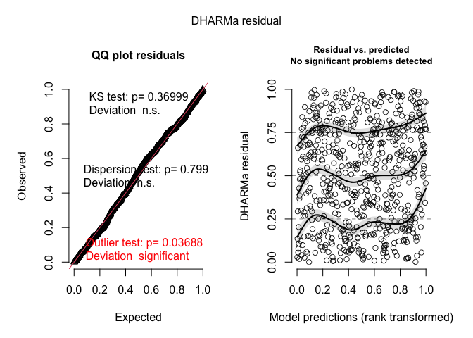
These diagnostic plots look pretty good (as they should since I
generated the data using an ordered probit model). If there were issues,
such as overdispersion, DHARMa would let you know with a lot of
scary looking red text.
Bayesian inference
While converting back to the probability scale using the thresholds
(intercepts) is a bit tricky, we actually don’t really need them for
some types of inference. In fact, we can still estimate things like the
probability that someone from the rural community rates the “natural”
picture higher than someone from the urban community, since this is
based on the linear predictor and doesn’t require the thresholds.
Furthmore, emmeans can make this inference pretty easy on us. To do
this, we need to get draws from the posterior distribution of the means
of interest, then compute how often one is larger than the other. Here
is an example.
post_draws <- as_draws_df(mfit_init, variable = "b", regex = T)
names(post_draws)
##  [1] "b_Intercept[1]"                  "b_Intercept[2]"
##  [3] "b_Intercept[3]"                  "b_Intercept[4]"
##  [5] "b_phototrails"                   "b_photobuildings"
##  [7] "b_communityurban"                "b_phototrails:communityurban"
##  [9] "b_photobuildings:communityurban" ".chain"
## [11] ".iteration"                      ".draw"
The first line in the above code block will extract any parameter with
“b” in it and add it as a column in a dataframe. This is useful since
brms uses “b” as a prefix for the “fixed effects” in the model. We can
now look at and create the posterior distributions of interest. In fact,
this first example comparing the difference in ratings between rural and
urban communities when shown the “natural” photo is captured by the
b_communityurban parameter.
ggplot(post_draws, aes(x = b_communityurban)) +
  geom_density()
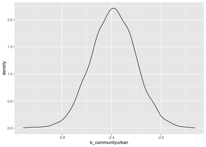
This provides the posterior density of the difference in means, rural-natural minus urban-natural. This suggests that there is a detectable difference between these two groups and that those from rural communities rate the “natural” photo higher, on average, than those from urban communities. The probability that someone from the rural community rate the “natural” photo higher than someone from the urban community is estimated to be
mean(post_draws$b_communityurban > 0)
## [1] 0
This is someone akin to a very small p-value for this contrast in frequentist statistics.
As a more complicated example, consider question of whether there is a difference in the average rating for photos “trails” and “buildings” between the two communities. This is how we could address that question:
post_q2 <- with(post_draws, {
  rural_trails <- 0 + b_phototrails
  rural_buildings <- 0 + b_photobuildings
  urban_trails <- 0 + b_phototrails + b_communityurban +
    `b_phototrails:communityurban`
  urban_buildings <- 0 + b_photobuildings + b_communityurban +
    `b_photobuildings:communityurban`
  # now do the means and difference of means
  0.5 * (rural_buildings + rural_trails) -
    0.5 * (urban_buildings + urban_trails)
})

mean(post_q2 < 0)
## [1] 0.99875
Thus, we estimate that the probability that the mean rating for photo “trails” and photo “buildings” for the rural community is less than the mean rating for the urban community is 0.99875.
Note that I included the 0s in the above calculations because the Intercept term, which is the mean for the rural-natural group, is fixed at 0.