Current Research
Bayesian learning methods for time series modeling
Long-term data collection on ecological systems can help to illuminate how a system evolves through time with both internal mechanisms (e.g., competition between species or predation) and in response to external perturbations (e.g., anthropogenic disturbance). Long-term ecological (LTE) data is also critically important for projecting future states of a system with climate change, landscape conversion, and management efforts. While the recognition of the utility of LTE data is widespread, we are still in early stages of processing and analyzing the accumulating data, and modeling techniques continue to evolve. For this project, we are interested in exploring the utility of Bayesian regularization and learning techniques in the analysis of LTE data with objectives of feature selection and forecasting.
Feature selection
Time series analysis often begins with a series of steps to detrend and remove seasonal cycles in the data in order to construct a stationary time-series. This process inevitably introduces some subjectivity since the researcher must decide which long lags to subtract to remove seasonality and which short lags to keep to yield a stationary time series. However, seasonal time series can also be described using an AR(\(p\)) model with \(p \to \infty\) and a sparse vector of AR coefficients \(\boldsymbol \phi\). Thus, given a sufficiently long time series, can we use Bayesian sparse learning techniques to fit the AR(\(p\)) model and bypass the differencing steps? This can also be extended to include arbitrarily many explanatory variables in the model.
Feature selection may also be useful in a variety of ecological contexts. Using a community ecology example, there is mounting evidence to suggest that competitive communities can be effectively described with models that lie somewhere between a fully parameterized model with unique competition coefficients for each species and one in which all species share the same competitive effect, resulting in a single competition coefficient (e.g., Skwara et al. 2023). Can we use unsupervised Bayesian learning techniques to efficiently collapse some competitive effects into a common, shared competition coefficient, while allowing estimates of different competitive effects for species that compete more strongly (Weiss-Lehman et al. 2022), and is there enough information in temporal fluctuations of species abundances to do so?
Forecasting
Regularization / parameter ‘shrinkage’, or adding constraints to the model fitting procedure such that some regions of parameter space are penalized and some are favored, can help to protect against model overfitting, or fitting the model too closely to the observed data such that out-of-sample predictions are poor. Most Bayesian learning techniques include strongly informative prior distributions that favor parameter values close to zero. This can result in parameter shrinkage that may improve model forecasts of future states in time series, especially if the length of the observed time series is short and the data are noisy, making overfitting more likely.
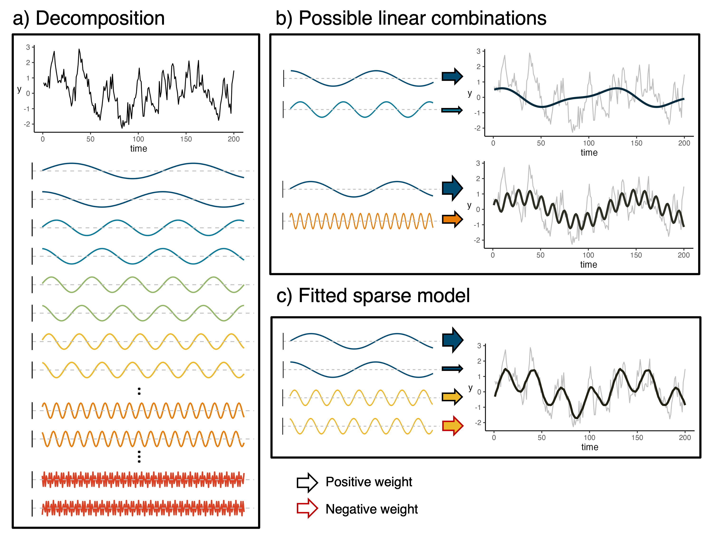
Forecasting may also sometimes be of interest even when data on potential covariates or drivers is not available. In this case, we are exploring the potential for Bayesian sparse modeling approaches to be applied as Bayesian smoothers to Fourier basis vectors. That is, we perform a change of basis with the data vector to a basis constructed with sine and cosine functions of increasing frequencies and use Bayesian learning techniques to smooth out the noise but keep the general trends in the data. This provides the potential for useful forecasts since the basis vectors, due to their construction with basic trigonometric functions, can be projected into the future.
Comparisons of sparse learning techniques
The development of sparse learning methods, or machine learning techniques that perform regression and model selection simultaneously, has exploded in recent years. Early versions of sparse regression include the Least Absolute Shrinkage and Selection Operator (LASSO; Tibshirani, 1996) and the similar (but not strictly sparse) Ridge regression, which both minimize the classic sum-of-squares loss function, but subject to constraints on the parameters. Specifically, the LASSO minimizes the loss function defined by \(L(\boldsymbol \beta) = ({\bf y} - {\bf X} \boldsymbol \beta)^\top ({\bf y} - {\bf X}\boldsymbol \beta) + \lambda ||\boldsymbol \beta||_1\) where \({\bf y}\) is the \(n\)-vector of responses, \({\bf X}\) is the \(n \times P\) model matrix, \(\boldsymbol \beta\) is the \(P\)-vector of regression coefficients, \(||{\bf v}||_1\) is the \(L_1\) norm of a vector \({\bf v}\), and \(\lambda\) is the penalty parameter. The \(L_1\) norm is equivalent to the sum of the magnitudes of all the elements in \(\boldsymbol \beta\), penalizing the loss function for increases in the magnitudes of the regression coefficients. I like to think of this as regression on a budget. If there are strong signals in the data, estimating those large parameters uses up much of the budget, forcing the remaining parameter estimates to shrink towards zero\(^*\).
Following these early developments and the recognition that the LASSO estimator is equivalent to the posterior mode estimate in a Bayesian regression in which the regression parameters are given independent Laplace priors (see Park and Casella, 2008), Bayesian sparse learning approaches have burgeoned in recent years. As a part of the Modelscape Consortium, an interdisciplinary and inter-institutional working group, my colleagues and I are comparing readily available software for different sparse modeling approaches. Specifically, we are interested in comparing:
- within- and out-of-sample predictive performance of the fitted models using software defaults
- Model selection accuracy (i.e., which elements of \(\boldsymbol \beta\) are zero and which are not?).
\(^*\)To see how the geometry of the LASSO penalty can force strictly sparse parameter vectors (those in which some parameters are estimated at exactly zero), check out my shiny app for this topic.
Missing data in data-driven time series models
The COVID-19 pandemic interrupted daily activities across the globe, including data collection (oh no!). In data-driven time series models, such as classical autoregressive models, missing data may be problematic because observations are both response and predictor. For example, assume observation \(Y_t\) is missing (denoting the missing data with capital letters and observed with lower-case) in a dataset to which we want to fit an AR(1) model. Ignoring the missing observation is problematic because we may violate the assumption of equal spacing between time points. Specifically, we wouldn’t want to fit the model \(y_{t+1} = \mu + \phi y_{t - 1} + \epsilon_{t + 1}\) when really our model is \(y_{t + 1} = \mu + \phi Y_{t} + \epsilon_{t + 1}\). Deleting all observations that involve the missing \(Y_t\) is also problematic because we have to delete more than just time point \(t\) as a response, but also \(t + 1\) since we have no predictor for \(t + 1\). With more than just one missing observation or an AR order of greater than 1, this widdles down a dataset rapidly.
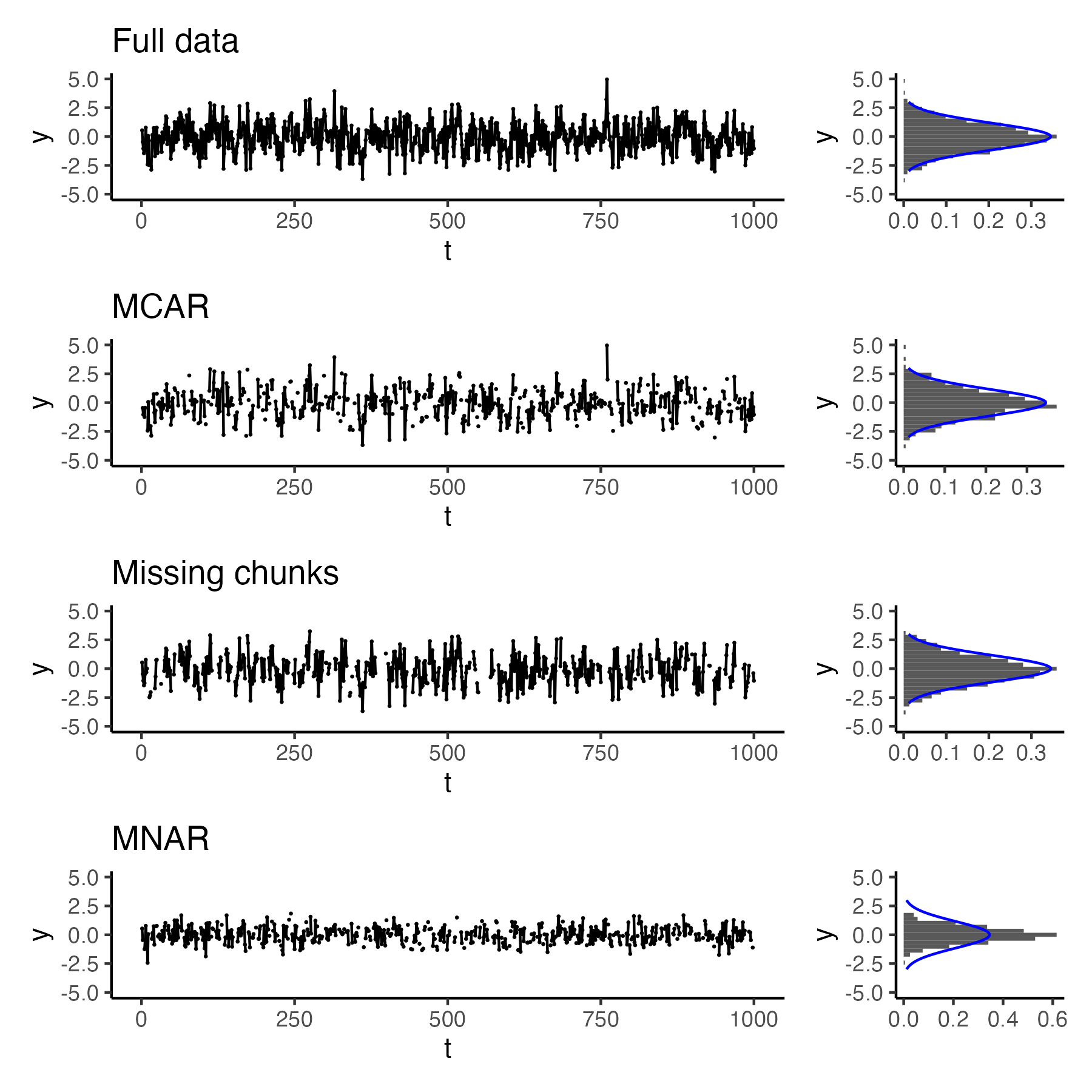
Along with others in the Modelscape Consortium, I am reviewing options for appropriately handling missing data in data-driven time series modeling for both Gaussian time series as well as time series of count data. We are comparing model fits to simulated data with different mechanisms for missingness (missing completely at random [MCAR], autocorrelated missingness that results in contiguous stretches of missing data, and missing not at random [MNAR] when extreme values are more likely to be missing) when using imputation techniques as well as model-based approaches such as Bayesian data augmentation and expectation maximization.